Informational Nodes: Plots

We can display any image at all in Cytoscape: we are not limited to the traditional simple shapes, text legends, simple borders and colors. The basic scheme is to:
  1. Create an image using your graphical tool of choice, and save it to a file.
  2. Give Cytoscape a URI saying where to find that file, and to which node it should be applied.

Because R is an exemplary environment in which to create data-driven graphics, RCy makes it easy to create and display expressive and detailed molecular maps.

Here is a simple example, a modest addition to our standard 'test and demo' RCy graph, which you can create via a call to makeSimpleGraph () (see 'methods'). There is an 
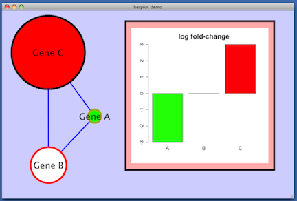
lfc attribute on the nodes, some made-up values (-3, 0, 3) which are used in this image to control the color of the nodes. Red indicates positive lfc, white is zero lfc, and green is negative lfc.


The first step is to develop and refine the custom graphics you want, working just in R: you don't want to display the custom graphics in Cytoscape until you are satisfied with them. (In addition, there appears to be a bug in Cytoscape 2.8.1 where you only get one chance to display a custom graphics. This 'sticks' and all subsequent images for a given node are ignored. I trust this will be fixed! If you need to replace a custom image you have placed on a network node, for now, unfortunately, you have to restart Cytoscape.).

For example: create a named list in R and display it as a barplot.

 
    lfc = c (-3, 0, 3) 
    names (lfc) =  c ('A', 'B', 'C')
    barplot (lfc, main='log fold-change', cex.main=2, cex.axis=1.5, cex.names=1.5, col=c ('green', 'white', 'red'))
When this looks right, write the image to a file rather than to the screen:
 
    lfc = c (-3, 0, 3) 
    names (lfc) =  c ('A', 'B', 'C')
    png ('barplot.png')
    barplot (lfc, main='log fold-change', cex.main=2, cex.axis=1.5, cex.names=1.5, col=c ('green', 'white', 'red'))
    dev.off ()
The final step is to tell Cytoscape to display this png file as the 'label' or 'face' of a specified node. More code and context are needed here; you might want to study these commands one line at a time, to make sure you see what each accomplishes. The broad steps are
  1. Create your graph. If you want your plot to be in an extra additional node, be sure to add that extra node to your graph.
  2. Create and display a CytoscapeWindow object containing that graph
  3. Render the graph, setting window size, layout, viz rules
  4. Create the custom graphics, here a barplot, save it to a file, then request Cytoscape to use it for the rending of your node
  5. redraw the screen, do a new layout
 
    window.title = 'barplot demo'
    g = RCytoscape::makeSimpleGraph ()
    g = graph::addNode ('lfc.plot', g)   # this is the new informational node
    nodeData (g, 'lfc.plot', attr='label') = 'plotting surface'  # give it a good label, later hidden by the plot
    cw = new.CytoscapeWindow (window.title, g)
    hideAllPanels (cw) 
    displayGraph (cw)
    layoutNetwork (cw, 'jgraph-spring')
    setWindowSize (cw, 800, 600)
    fitContent (cw)
    setZoom (cw, 0.9 * getZoom (cw))

    setNodeLabelRule (cw, 'label')
    node.attribute.values = c ("kinase",  "transcription factor")
    colors =                c ('#A0AA00', '#FF0000')
    setDefaultNodeBorderWidth (cw, 5)
    setNodeBorderColorRule (cw, 'type', node.attribute.values, colors, mode='lookup', default.color='#000000')
    count.control.points = c (2, 30, 100)
    sizes                = c (20, 50, 100)
    setNodeSizeRule (cw, 'count', count.control.points, sizes, mode='interpolate')
    setNodeColorRule (cw, 'lfc', c (-3.0, 0.0, 3.0), c ('#00FF00', '#FFFFFF', '#FF0000'), mode='interpolate')
    redraw (cw)

    lfc.values = noa (g, 'lfc') [1:3]  # don't pick up the fourth node -- that's the informational one!
    png ('barplot.png')
    barplot (lfc.values, main='log fold-change', cex.main=2, cex.axis=1.5, cex.names=1.5, col=c ('green', 'white', 'red'))
    dev.off ()
       # the image file is, for now, in your working directory, with the name you gave it

    setNodeImageDirect (cw, 'lfc.plot', sprintf ('file://%s/%s', getwd (), 'barplot.png'))
    setNodeSizeDirect (cw, 'lfc.plot', 200)
    layoutNetwork (cw, 'force-directed')
    redraw (cw)

Further Comments

  1. If you save your network as a Cytoscape session file, you have to move your image files to a universally visible URI. For instance,
     setNodeImageDirect (cw, 'lfc.plot', 'file://data/proj/barplot.png') 
    must become
     setNodeImageDirect (cw, 'lfc.plot', 'http://server.xyz.com/data/proj/barplot.png') 
    When your network attains some stability, and you are ready to publish it more widely, you can move all your images to a webserver, regenerate the Cytoscape session from your R script, and then save the .cys file; the http-based uri's will be used and stored in the session file, making the image-laden network usable everywhere.

  2. The example above adds a separate 'informational' node to the graph; none of the original 'data' nodes of the graph are changed. You can just as easily put custom images on some or many of your data nodes. For instance, if you have a time course experiment, with expression measured at each timepoint, you could create a graph of each gene's expression over time, and have those x-y plots be the rendered nodes displayed by Cytoscape.